▶ Cinematic fable · Watch on YouTube ▶ 影片版寓言 · 在 YouTube 观看
镇上有一间老邮局,只有一个柜台。
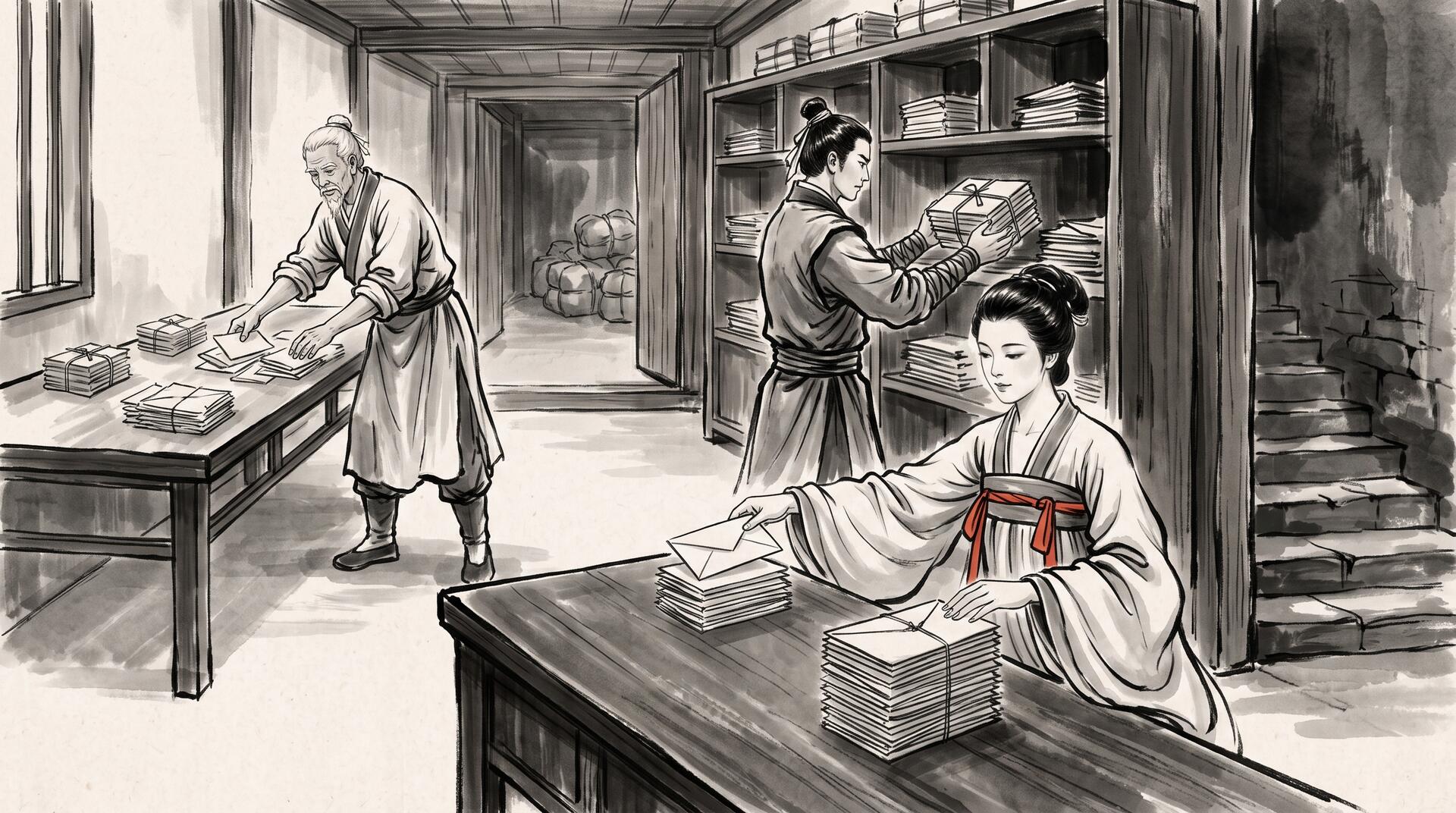
每天镇民送来的信和包裹络绎不绝。邮局的规矩很特别:柜台后面坐着一位年轻的收件员,面前放着一张大桌子。每封信到了,收件员不急着往后面搬,而是按寄件人的姓氏顺序插进桌上的信堆里——桌面上永远保持着排好序的一摞。查信的人来了,先翻桌上这摞,几秒钟就能找到。
但桌子有限。信堆涨到大约两百封的时候,收件员把整摞信用绳子一捆,写上编号,递给身后的助手。助手把这一捆放到”近期架”上——一排靠墙的木架子。近期架上可以摆好几捆,每捆内部都是排好序的,但捆与捆之间并没有统一排序。
隔一阵子,近期架也会满。这时候邮局里一位老档案员出场了。他把近期架上的几捆信全搬下来,摊在长桌上,像玩扑克牌一样把它们归并成一大捆——姓氏相同的信只留最新的那封,旧的丢进废纸篓。归并好的大捆被搬进走廊尽头的储藏室。储藏室里的捆更大、更老、查得更慢,但每一捆里面的信仍然是严格排序的。
要是储藏室也快满了怎么办?地下室还有一层更深的档案架。老档案员会把储藏室的几大捆再归并一次,搬到地下室。地下室的捆最大、最老、查得最慢——但只要你知道在哪一层,顺着排序一翻就行。
来查信的镇民不知道这些层级。他只需要告诉收件员”我找王记铁铺的信”,收件员就按顺序找:先翻桌面(最快)、再翻近期架上的每一捆、再翻储藏室、最后翻地下室。大多数时候桌面或近期架就能找到。
后来助手想了个省事的法子:每一捆信封好之前,他用一张小卡片记下”这一捆里绝对没有哪些姓氏”。查信时先瞄一眼小卡片,上面说没有王记,就跳过这捆,不用拆开翻了。省下的时间相当可观。
镇民们有时候纳闷:写入这么快,查找偶尔要翻好几层,会不会慢?老档案员笑着说,诀窍在于写的时候永远只往桌上加,绝不回头改老捆。改老捆要拆绳、抽信、重新捆——那才是慢的。只要定期归并,老捆里的废信就自然被清掉了。
——到这儿你大概已经认出来了:这就是 LSM tree(Log-Structured Merge-tree)。
这是什么
LSM tree 是一种为写密集型场景设计的数据结构。新写入先进入内存中的有序缓冲区(memtable)。当 memtable 满了,它被整体刷写(flush)成磁盘上的一个不可变有序文件,叫 SSTable(Sorted String Table)。多个 SSTable 在磁盘上分层堆积(Level 0, Level 1, …),每一层容量更大。后台的 compaction 过程会把同一层的多个 SSTable 归并成下一层的更大 SSTable,同时丢弃过期或被覆盖的记录。
读取时,从 memtable 开始,依次往更深的层级查找,直到找到目标 key。每个 SSTable 可以附带一个 Bloom filter,快速判断某个 key 是否不在这个文件里,从而跳过无关文件。
为什么重要
RocksDB、LevelDB、Cassandra、HBase、CockroachDB——几乎所有现代写密集型存储引擎的核心都是 LSM tree。它把随机写变成顺序写(只做 append 和归并),让写吞吐量可以逼近磁盘顺序 I/O 的上限。代价是读可能需要查多层,以及 compaction 会消耗 CPU 和 I/O 带宽。调优 LSM 本质上就是在写放大、读放大、空间放大之间做 tradeoff——Leveled compaction、Tiered compaction、FIFO compaction 各有取舍。Kubernetes 的 etcd 底层用的就是 BoltDB(B+ tree),而不是 LSM;但如果你运行 Cassandra 或 CockroachDB 的 workload,理解 LSM 的 compaction 行为直接决定了你能不能诊断写延迟毛刺和磁盘 I/O 风暴。
隐喻对应表
- 收件员的桌面,信按姓氏排好序 → 内存中的 memtable,有序缓冲区
- 桌满了用绳子捆好递给助手 → flush,memtable 刷写成 SSTable
- 近期架上的一捆捆信 → Level 0 的多个 SSTable
- 老档案员把几捆归并成一大捆 → compaction,归并多个 SSTable
- 归并时丢掉重复的旧信 → compaction 丢弃过期/被覆盖的记录
- 储藏室、地下室 → 更深的层级(Level 1, Level 2, …)
- 查信时从桌面开始、逐层往深处找 → 读路径从 memtable 到 L0 到 L1…
- 小卡片记”这捆没有哪些姓氏” → Bloom filter,快速跳过无关 SSTable
- 写入只往桌上加,不拆老捆 → 只做 append,避免 random write
- 定期归并清废信 → compaction 回收空间、降低读放大
There is an old post office in the town, a single counter.
Letters and parcels arrive all day. The post office has a peculiar system: behind the counter sits a young clerk with a wide desk. When a letter arrives, the clerk does not carry it to the back room right away. Instead, she slides it into the sorted stack on her desk — filed by the sender’s surname, always in order. Anyone who comes to look for a letter checks the desk first; it takes only seconds.
But the desk is finite. When the stack grows to roughly two hundred letters, the clerk ties it with twine, writes a serial number on the bundle, and hands it to an assistant behind her. The assistant places the bundle on the “recent shelf” — a row of wooden racks against the wall. The recent shelf can hold several bundles. Each bundle is internally sorted, but the bundles themselves are not sorted relative to one another.
After a while, the recent shelf fills up too. That is when the old archivist steps in. He pulls every bundle off the recent shelf, spreads them on a long table, and merges them the way you merge runs of playing cards — for any sender that appears more than once, only the newest letter is kept; the rest go into the wastepaper basket. The merged super-bundle is carried to the storeroom at the end of the corridor. Storeroom bundles are larger, older, and slower to search, but the letters inside each one are still in strict order.
If the storeroom fills up? There is a cellar with an even deeper set of racks. The archivist merges storeroom bundles once more and moves them down. The cellar bundles are the biggest, the oldest, and the slowest to search — but as long as you know which level you are on, you can flip through the sorted letters quickly enough.
A townsperson looking for a letter knows none of this. She simply tells the clerk “I need the letter from Wang’s Ironworks,” and the clerk searches in order: desk first (fastest), then each bundle on the recent shelf, then the storeroom, then the cellar. Most of the time, the desk or the recent shelf is enough.
The assistant eventually came up with a shortcut: before sealing each bundle, he jots down on a small card which surnames are definitely not inside. When searching, a glance at the card — “no Wang here” — and the bundle is skipped without being untied. The time saved is considerable.
Townspeople sometimes wonder: writes are so fast, but reads might have to dig through several levels — won’t that be slow? The old archivist smiles and says the trick is that writes only ever add to the desk; they never go back and amend an old bundle. Untying a bundle, pulling a letter out, re-sorting, re-tying — that is what’s slow. As long as you merge regularly, the dead letters in old bundles get cleaned out naturally.
— By now you’ve probably recognized it: this is the LSM tree (Log-Structured Merge-tree).
What it is
The LSM tree is a data structure designed for write-heavy workloads. New writes land first in an in-memory sorted buffer called the memtable. When the memtable fills, it is flushed as a whole into an immutable sorted file on disk called an SSTable (Sorted String Table). Multiple SSTables accumulate on disk in layers (Level 0, Level 1, …), each layer holding progressively more data. A background compaction process merges SSTables from one level into larger SSTables at the next level, discarding stale or overwritten records along the way.
Reads start at the memtable and work downward through the levels until the target key is found. Each SSTable can carry a Bloom filter — a probabilistic data structure that can quickly say whether a key is definitely not in that file, allowing the reader to skip irrelevant files entirely.
Why it matters
RocksDB, LevelDB, Cassandra, HBase, CockroachDB — nearly every modern write-heavy storage engine is built around LSM trees. The structure turns random writes into sequential writes (only appends and merges), pushing write throughput close to the disk’s sequential I/O ceiling. The tradeoff is that reads may need to probe multiple levels, and compaction consumes CPU and I/O bandwidth. Tuning an LSM engine is fundamentally about balancing write amplification, read amplification, and space amplification — Leveled compaction, Tiered compaction, and FIFO compaction each make different bets. Kubernetes’ etcd uses BoltDB (a B+ tree), not an LSM; but if you run Cassandra or CockroachDB workloads, understanding LSM compaction behavior is what lets you diagnose write-latency spikes and I/O storms.
Metaphor mapping
- the clerk’s desk, letters sorted by surname → the in-memory memtable, a sorted buffer
- tying the full stack and handing it back → flush, memtable written to an SSTable
- bundles on the recent shelf → multiple SSTables at Level 0
- the archivist merging bundles into a super-bundle → compaction, merging SSTables
- discarding duplicate old letters during merge → compaction dropping stale/overwritten records
- the storeroom and cellar → deeper levels (Level 1, Level 2, …)
- searching desk first, then each deeper level → read path from memtable through L0, L1, …
- the card listing which surnames are “definitely not here” → Bloom filter, skipping irrelevant SSTables
- writes only add to the desk, never amend old bundles → append-only writes, no random updates
- regular merging clears dead letters → compaction reclaims space and reduces read amplification